Overview

Teaching: 20 min
Exercises: 20 min

Questions

• How can observations be checked for errors given dates or transcriptions?

Objectives

• Animate by collecting event date or collector to show biases in collection.

Are there biases in the collection by collector or errors with dates or transcriptions? Which points were collected by the same collector or have low data quality scores? (For all records before 1940, what institutions? - by institution code), bias based on institutional protocols - build a query

• Goal: visually assess data quality or outliers
• Tool: TimeManager (requires installation of Plugin; go to Manage and Install Plugins and search) - warning: this dataset is very large, so running TimeManager can be somewhat slow
• Output: same layer with time enabled symbology for attribute of interest

Toggle on TimeManager Plugin from the menu; this will open the interactive panel.

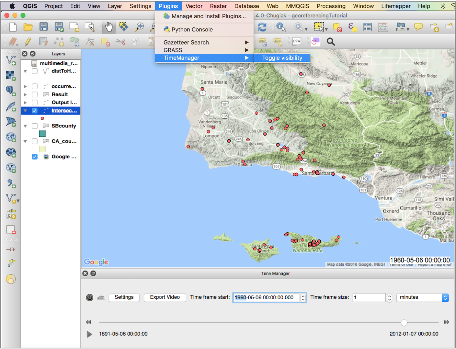
Choose a time field (i.e. dwc:dcterms_mo, dwc:eventDate, dwc:year) from the “occurrences_raw.csv” to use as a timestamp. You can choose a start time of interest and see which observations correspond to this start date. This is another means of revealing patterns in your symbolized data.

Centroids

Are the observations georeferenced to a county or state level?

• Goal: find points that are not descriptively georeferenced
• Tool: Polygon centroids; (Dissolve)
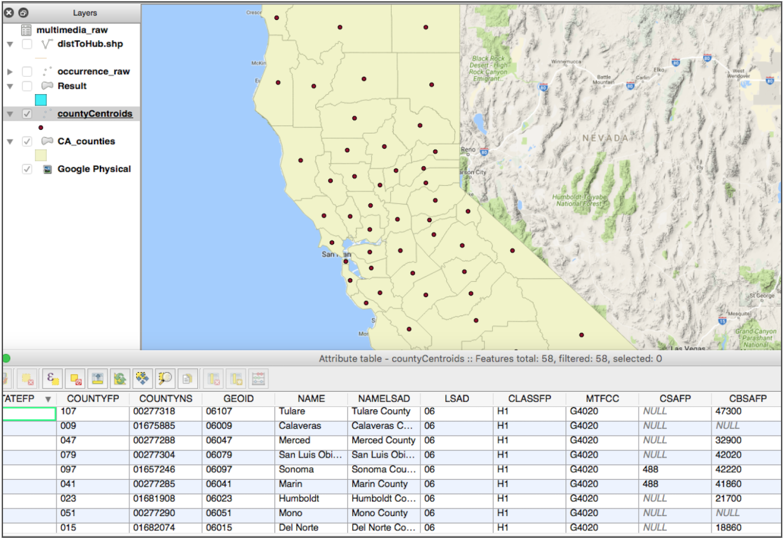
• Output: a new shapefile with points that describe the geometric center of each polygon

Open the Polygon centroids tool from the processing toolbox. Use the CA Counties layer as your input and save out the centroids to a new shapefile in your same folder directory.

Buffer

What is the acceptable distance from the centroid as a proxy measure of granularity?

• Goal: find points that are within an acceptable threshold distance from the centroid of the counties
• Tool: Buffer(s)
• Output: a new shapefile of polygons with areas of a given search radius around each centroid

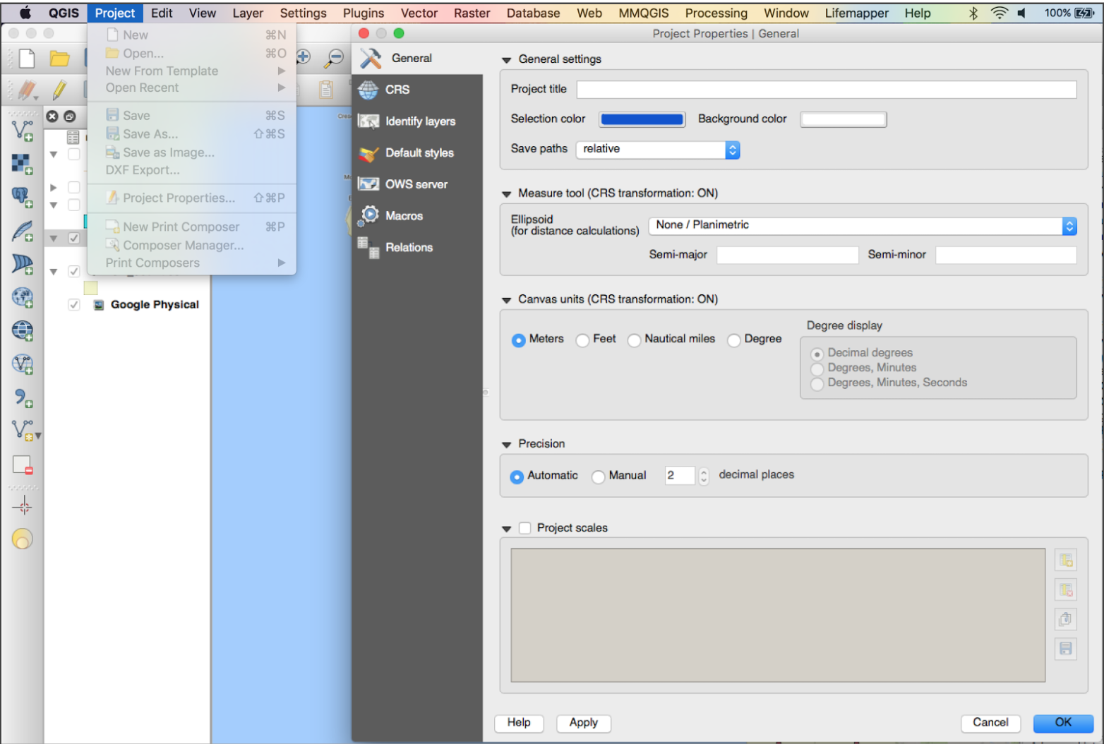
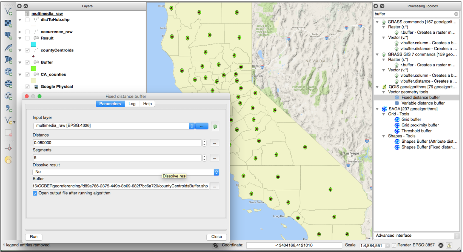
Open the Fixed Distance Buffer tool from the processing toolbox. You are prompted to select a Buffer distance. To find out the project properties and units, navigate to Project > Project Properties > General. You will see that CRS transformation is enabled (your layers are projected on the fly) and your canvas map units are in Meters. Your projection is Pseudo Mercator, so your map units are in Decimal Degrees.

As a first pass, generate a 0.08 degree buffer (approximately 5.5 miles) around each centroid. Since this is a proxy measure for granularity, you can choose any buffer radius that makes sense.

Intersect

Do any observation points Intersect the buffer? If so, is the precision of these observations suspect?

• Goal: find points that intersect the threshold distance
• Tool: Intersect
• Output: a selection of points (highlighted in the attribute table) that intersect the search radius

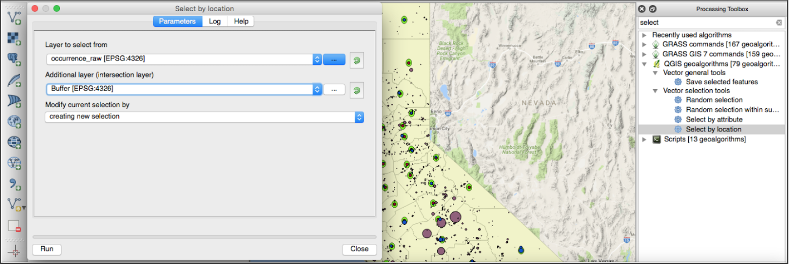
Find the Select by Location tool in the Processing Toolbox. Specify the occurrences_raw.csv points as the layer to select from and the Buffer as the intersection layer.

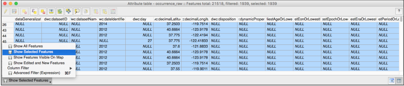
We can now review the 1939/21518 subset of occurrences that are geocoded to within a 5 mile radius of the county centroid. Filter in the attribute table to sort “Show Selected Features”. At the top of the table, the number of selected features is reported. Review the Longitude and Latitude of the coordinates and note the precision. Is it spurious? What is the date of the record?

Key Points