Overview

Teaching: 30 min
Exercises: 30 min

Questions

• What is the difference between vector and raster data?

Objectives

• Set up QGIS and load data.

• Preview and explore toolkits.

Load data

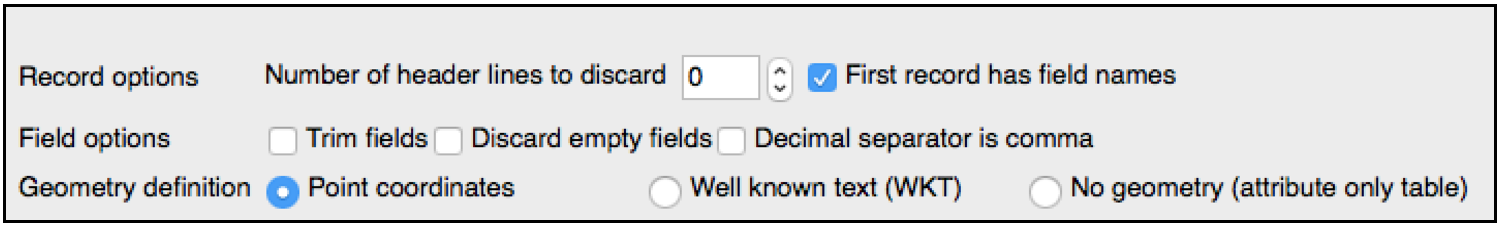
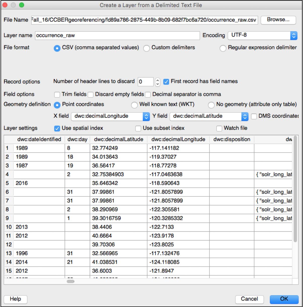
Load the occurrence_raw.csv in QGIS as a delimited text layer. The data are comma separated. Specify your Longitude field as your X and your Latitude field as your Y. Ensure that the ‘discard empty fields’ box, remains unchecked, as selecting it will collapse column formatting.

• Note: The X and Y coordinates are easily confused. Latitude specifies the north-south position of a point and hence it is a Y coordinate. Similarly, Longitude specifies the east-west position of a point and it is a X coordinate. If prompted to select a CRS (coordinate reference system), select WGS84 (default), which will allow for combination with other layers using the same reference.

Set projection

Check the CRS if you see an error stating that the Coordinate Reference System is undefined. Once the layer is imported, right click on it and go to Properties > General. Check the CRS here.

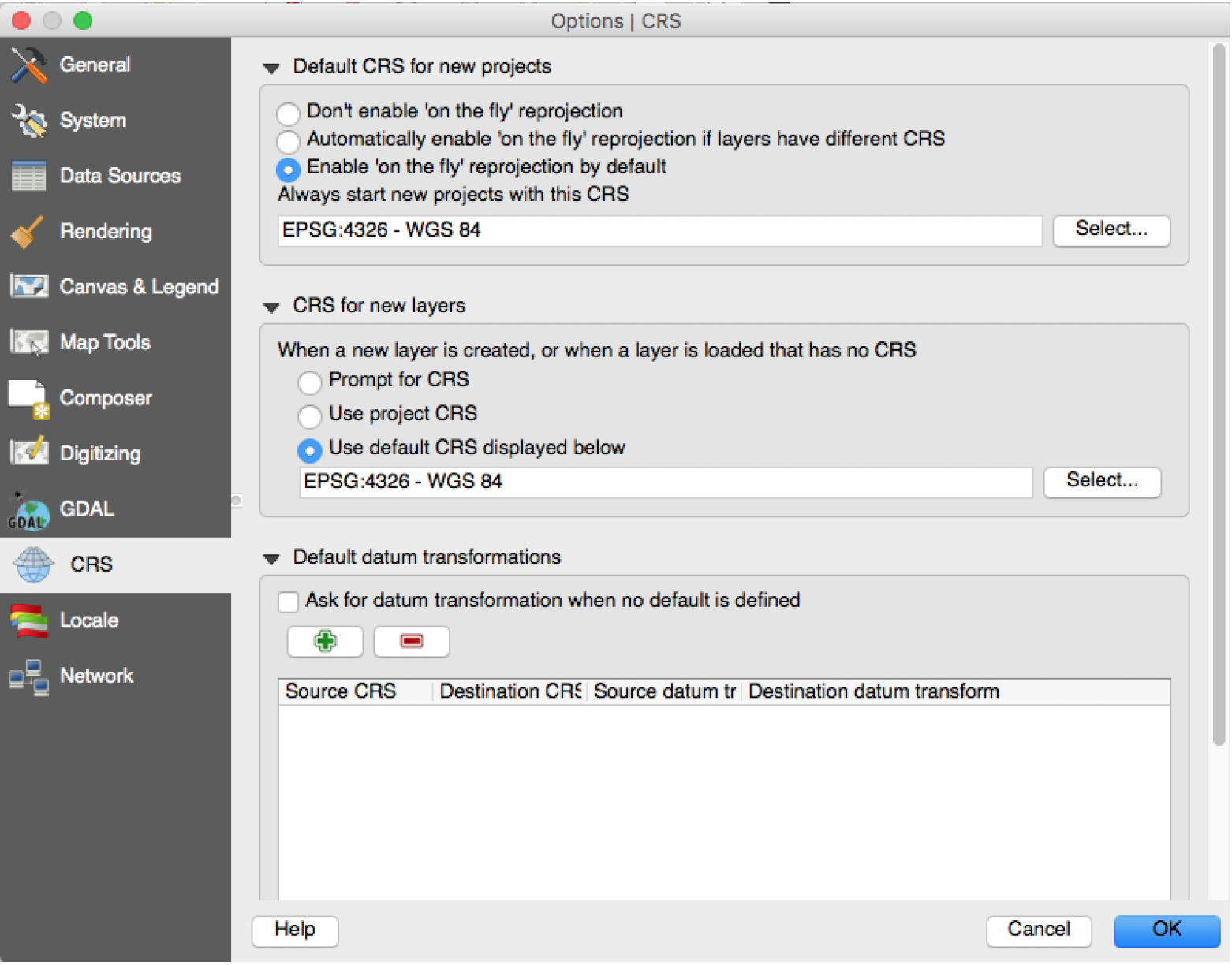
Set the QGIS > Preferences for CRS (coordinate reference system) to Enable on the Fly reprojection by default. Your data may be projected to WGS:84 by default. This is a very standard datum (for WGS84 pseudo mercator for web). In order to analyze your points against other data layers, you may need to change the CRS (vector) or reproject/warp (raster) those layers into WGS84, etc. Always check the CRS of the layers that you import to ensure that they are aligned.

Style points

Change the appearance of points by right-clicking on the layer in the legend and selecting Properties. Within the Style pane, you can change the Color and Size of the points according. It is also through this panel that you also can symbolize the points based on an attribute or scale their radius proportionally.

Preview attributes

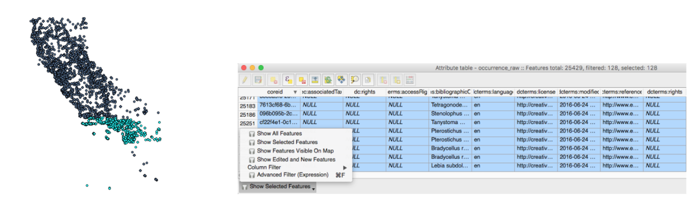
Open the attribute table by right-clicking on the layer and selecting Open Attribute Table. There are 25,429 features! Selecting a row(s) in the attribute table will highlight the respective point(s).

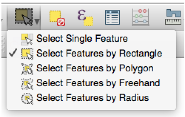
Change the selection highlight color under Project > Project Properties in the Canvas & Legend Panel under selection color. This will highlight the selected features on your map. You can interactively select data by cursor clicking on the map or dragging a rectangle around points.

This will highlight the records in the corresponding attribute table. In the table, you can toggle between viewing all records and viewing the selected records. To create a subset of data points, you can manually select records and see the corresponding records in the attribute table.

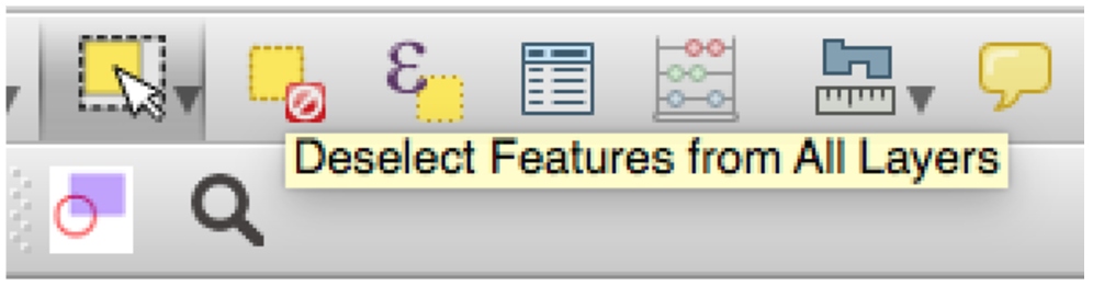
To clear your selection, hit Deselect Features from All Layers.

Load supplementary data

Load the supplementary California Counties (shapefile) layer that you downloaded from Box. You do not have to unzip this shapefile. Shapefiles are actually bundles of 6-8 composite files, but QGIS can read this in as one package when imported. Also check the CRS information for the layer by right clicking to Properties > General. It is in the same CRS as the points (WGS84).

• To import vector layers (i.e. shapefiles):

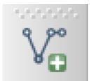
• To import raster layers (i.e. tiffs):

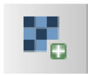
• To import text delimited layers (i.e. spreadsheets):

Style layers

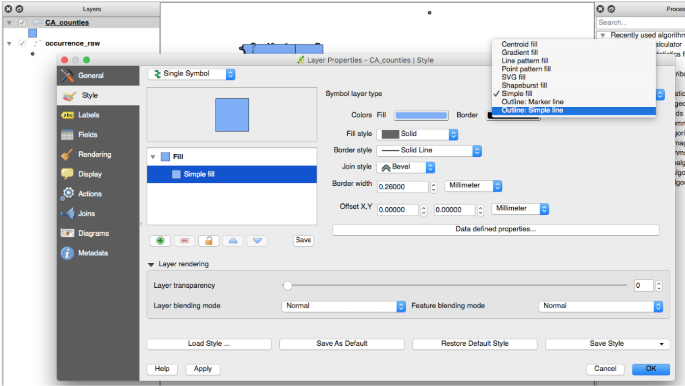
Change the appearance of the CA_counties in Properties. You can change the symbology of the layer to render it transparent or hollow, which will allow you to layer it with other content. Right-click on the CA_counties layer and go to Properties > Style. Rather than a Simple fill, the style can be Outline: Simple line, which will render the layer as hollow. Hit Apply to preview the change in the canvas and hit Ok once you are satisfied with the Style.

Drag the CA_counties layer beneath the points to change the order. You can also check or uncheck the box next to the layer name to toggle the layer on or off.

Explore data

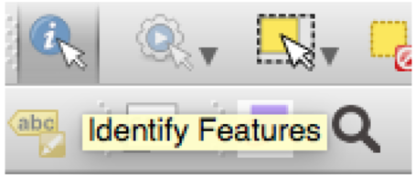
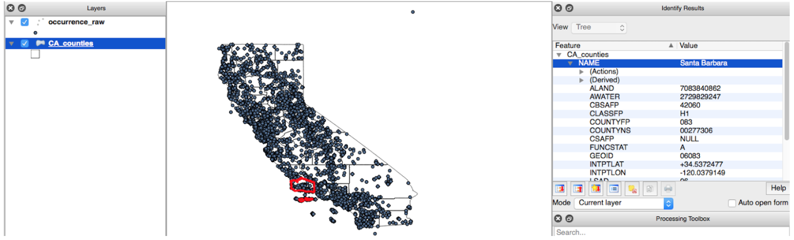
Interrogate the data by using the Identify tool. Depending on the layer selected (points or counties), you can click on the feature in the canvas of interest and see its attributes. Click away from features on the canvas to deselect.

Load a basemap of your choice from Web > OpenLayers plugin, preferably from OpenStreetMap. You can see the points referenced against tiled basemaps (physical, streets, etc)

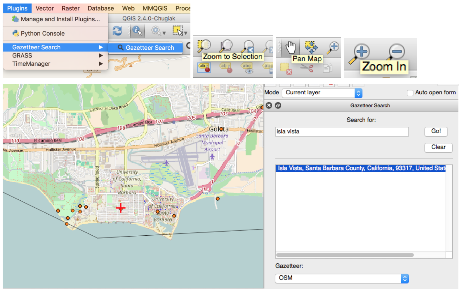
• If you don’t see this option, go to Plugins > Manage Plugins and ensure that the OpenLayers box is checked on.

Explore the data by place name with the Gazetteer plugin. Search for places (i.e. “botanic gardens California”, etc.) and note the distribution of points around each. Zoom using the magnifying glass and pan with the hand icon.

Save project

Save your map project. Now that you have loaded your georeferenced data points, the California Counties, and a basemap of your choice, be sure to save a project file (.qgs) so you can reopen your records again later. Be sure to continue storing all of your content, including the project file and layers that you load and produce, in the same working directory folder.

• Note: The project file (.qgs) does not save any of the data. Rather, it stores the relative file paths for the layers that comprise the project and preserves the cosmetic appearance of the layers, such as the symbology and order of the layers in the project. This means you can close out your project and later return to it by launching the project file; your layers and symbology are preserved and remain as you saved them, provided you do not change the locations of the project layers.

Key Points