Overview

Teaching: 35 min
Exercises: 40 min

Questions

• What kinds of auxiliary data can complement spatial analysis?

Objectives

• Add auxiliary data layers.

• Save maps and data.

Add additional layers

Add additional layers of interest, which you downloaded (and are also linked to their sources below): EPA Ecoregions Level III (shapefile); National Park Boundaries (shapefile); Natural Earth Shaded Reliefs (raster: available in large, medium, and small scale). We can use these in analysis.

• Note: You can also search for other thematic layers that might be of particular interest to your project using ArcGIS Online. Additional ideas for supplementary data include imagery: vegetation, land cover, natural preserve boundaries, or roads. These layers can provide context for the research questions that you would like to answer.
• Note: Depending on the size of the study area you’re interested in, you may want to examine the resolution of the elevation data cells to assess their utility. Examining county-level data for instance requires finer resolution grid cells, compared with data of national extent.

Save layers

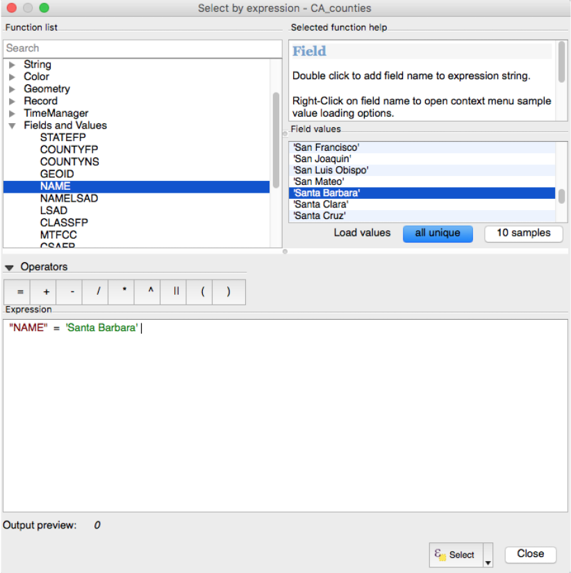
Save a single feature as a separate layer, such as the county of Santa Barbara. Make a selection, either in the attribute table or by making a selection on the map. Right-click the CA_Counties layer in the legend and select Save Vector Layer As. We can also build a query expression from the County attribute table to select California.

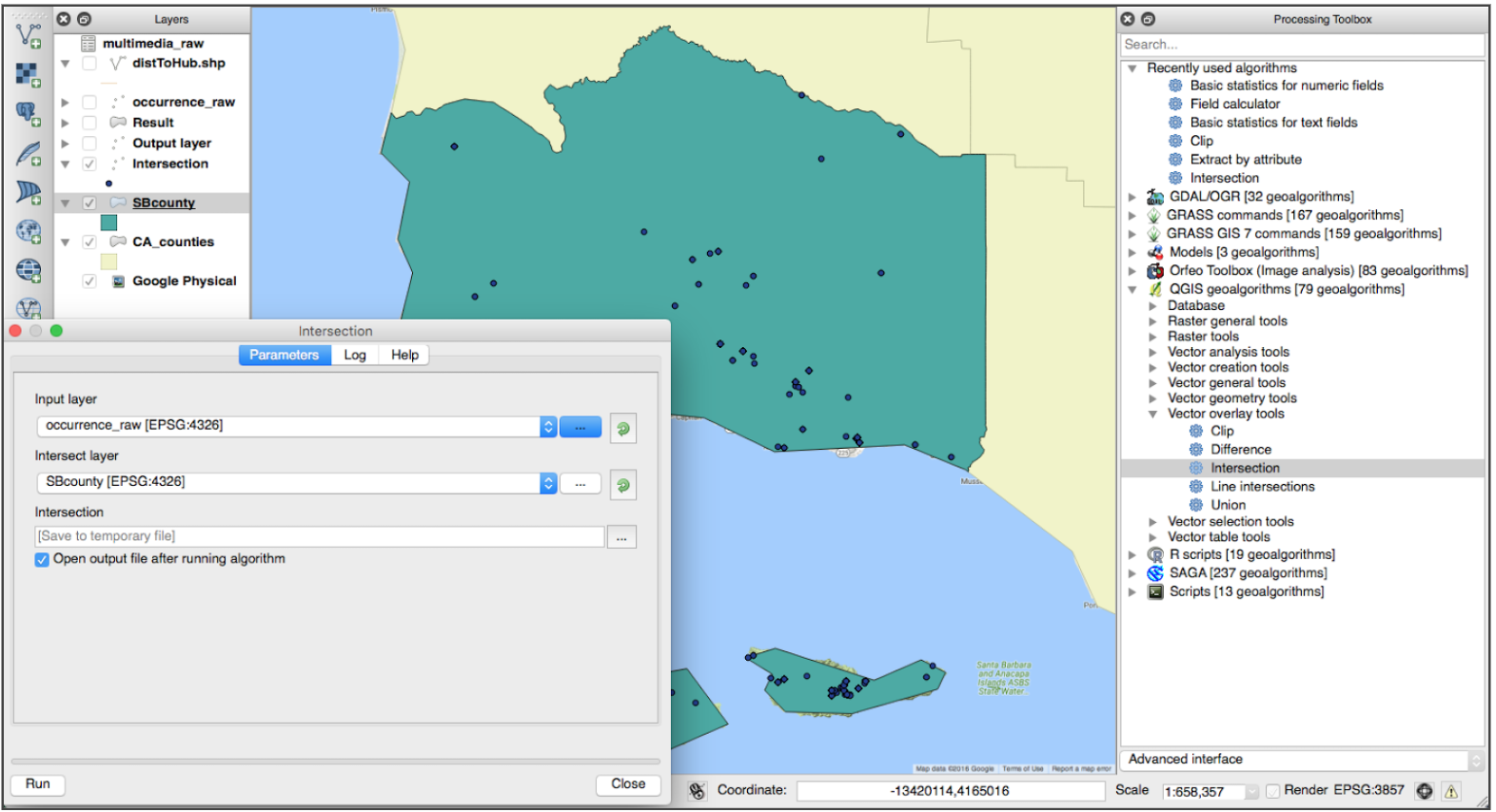
Create a subset of observations within the county by using the Intersection tool. You will need to open the Processing toolbox from the Processing dropdown menu. Select the occurrences_raw as the input layer and Santa Barbara County as the intersect layer. You can write the intersection of the layers to a new file by specifying a filepath and name. Once the tool runs, hit Close.

Share map

To share your map with others, you have several options for export. You can zip your project folder to send your QGIS project, or export the project to print as a PDF from the Project > Save as Image or in Composer, which allows for more advanced cartographic styling. You can also save a frame from your canvas under Project > Save as Image as any image type you wish.

Join media

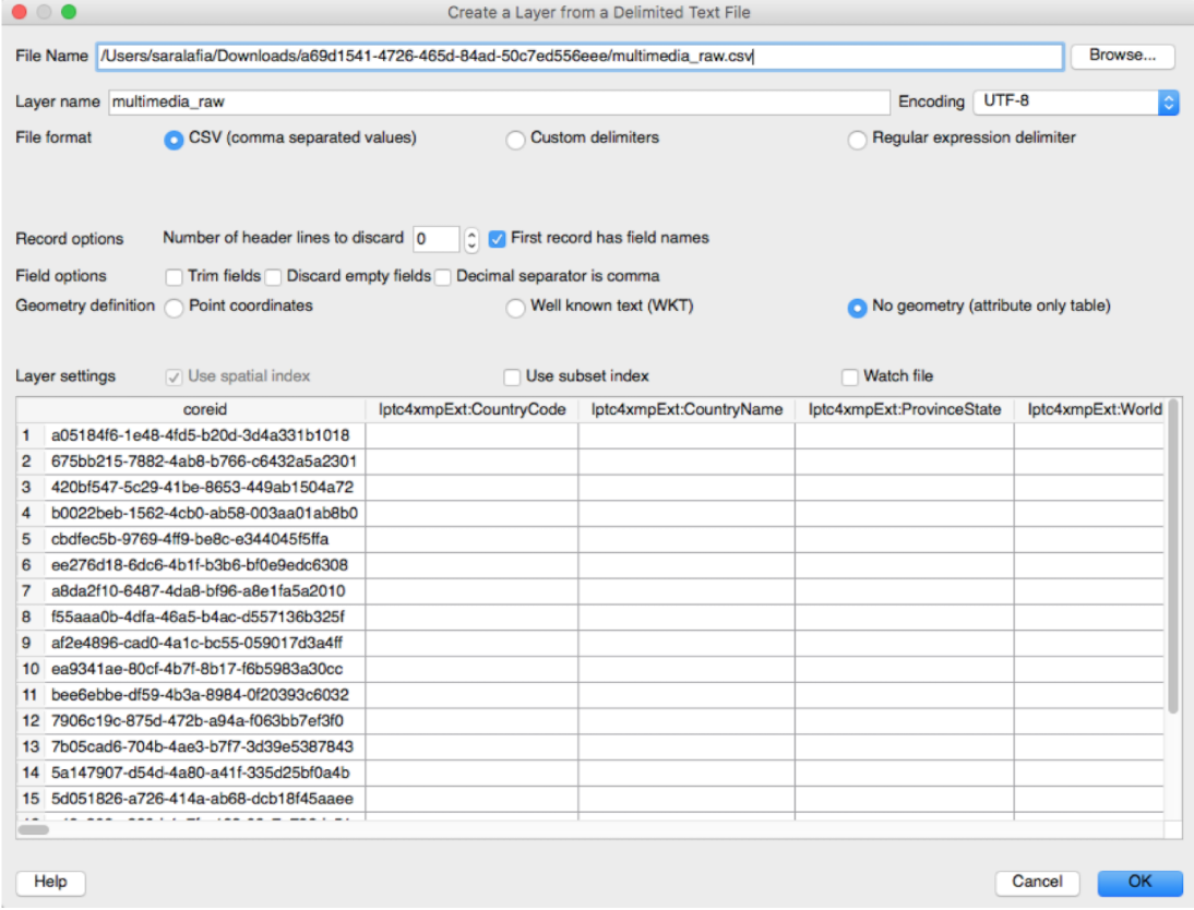
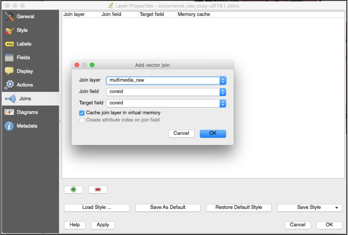
Join the multimedia.csv table to your occurrence table using idigbio:coreid as a primary key. This is the unique identifier of the dataset records, analogous to the idigbio:UUID. Import the table as you imported occurrences_raw and create a layer from delimited text and indicate “No Geometry”, loading the table just as an attribute table. Many records point to access URIs that contain media, such as photographs associated with the point. Remember to keep saving your project periodically!

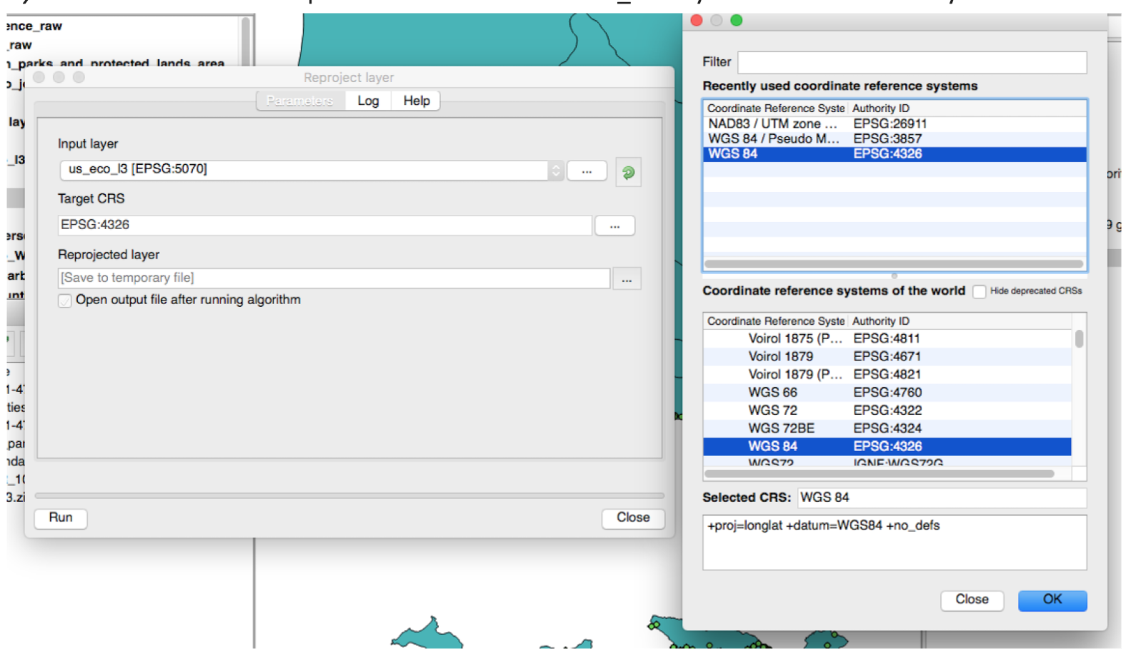
Reproject the Ecoregions layer from NAD83 to WGS84 using the Vector general tools > Reproject layer. This will make it interoperable with the occurrences_raw layer and other WGS84 layers.

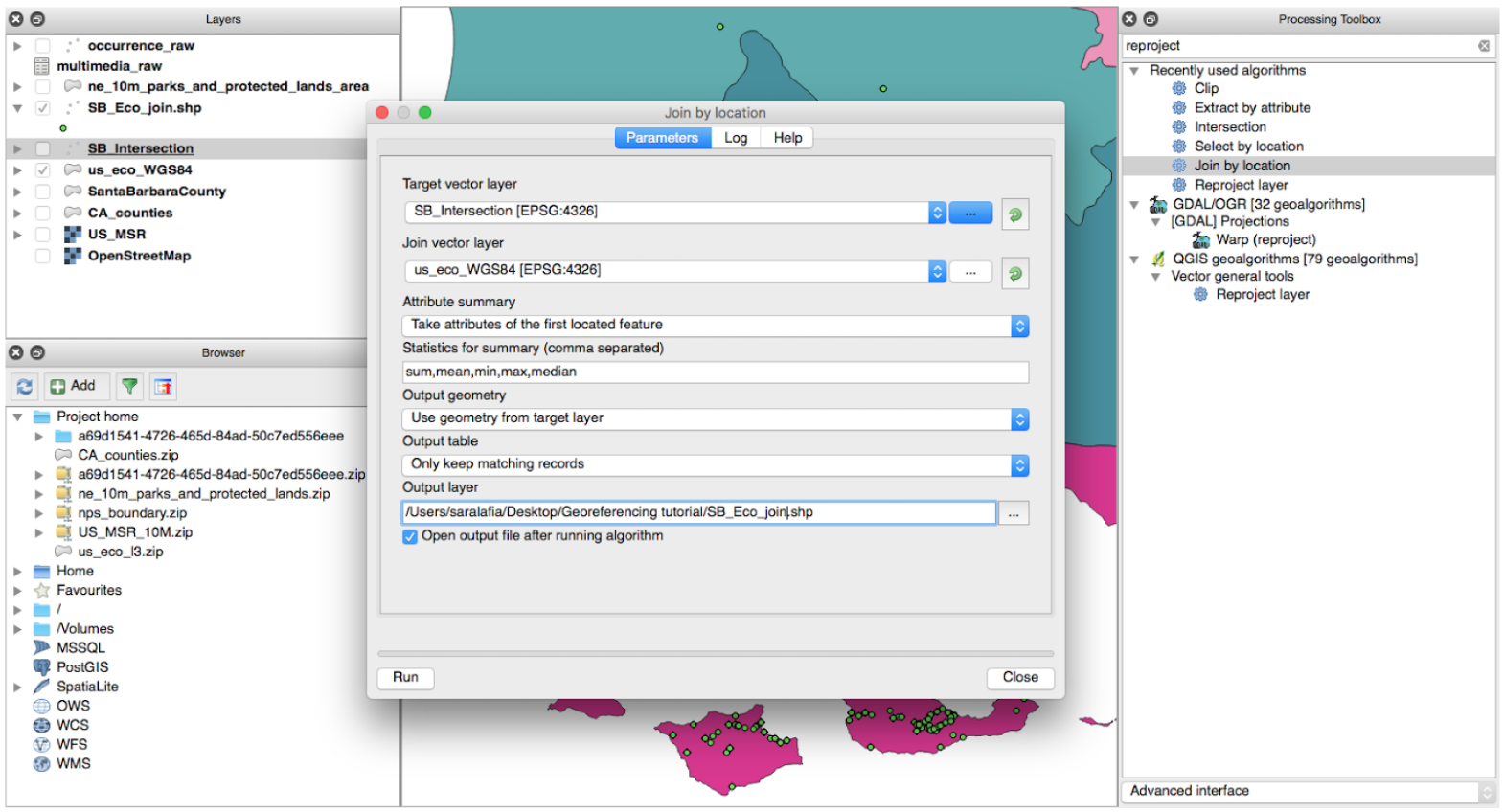
Join by location using the Vector General Tools > Join by Location to get the US Ecoregions attribute table (join vector layer) joined with the occurrences within Santa Barbara (target vector layer). This will append the attribute table of the Ecoregions layer to the occurrences points.

Shortcut

The entire zipped QGIS project to this point is available for download here (launch Tutorial.qgs).

Key Points