R for reproducible scientific analysis

Multi-Table Joins

Learning objectives

Focus on the third tidy data principle
- Each variable forms a column.
- Each observation forms a row.
- Each type of observational unit forms a table.
By able to use dplyr’s join functions to merge tables

Joins

The third tidy data maxim states that each observation type gets its own table. The idea of multiple tables within a dataset will be familiar to anyone who has worked with a relational database but may seem foreign to those who have not.

The idea is this: Suppose we conduct a behavioral experiment that puts individuals in groups, and we measure both individual- and group-level variables. We should have a table for the individual-level variables and a separate table for the group-level variables. Then, should we need to merge them, we can do so using the join functions of dplyr.

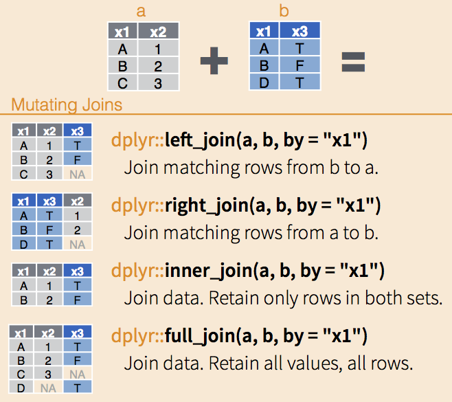
The join functions are nicely illustrated in RStudio’s Data wrangling cheatsheet. Each function takes two data.frames and, optionally, the name(s) of columns on which to match. If no column names are provided, the functions match on all shared column names.

The different join functions control what happens to rows that exist in one table but not the other.

left_join keeps all the entries that are present in the left (first) table and excludes any that are only in the right table.
right_join keeps all the entries that are present in the right table and excludes any that are only in the left table.
inner_join keeps only the entries that are present in both tables. inner_join is the only function that guarantees you won’t generate any missing entries.
full_join keeps all of the entries in both tables, regardless of whether or not they appear in the other table.

dplyr joins, via RStudio

We will practice on our continents data.frame from module 2 and the gapminder data.frame. Note how these are tidy data: We have observations at the level of continent and at the level of country, so they go in different tables. The continent column in the gapminder data.frame allows us to link them now. If continents data.frame isn’t in your Environment, load it and recall what it consists of:

load('data/continents.RDA')
continents

   continent area_km2 population percent_total_pop
1     Africa 30370000 1022234000              15.0
2   Americas 42330000  934611000              14.0
3 Antarctica 13720000       4490               0.0
4       Asia 43820000 4164252000              60.0
5     Europe 10180000  738199000              11.0
6    Oceania  9008500   29127000               0.4

We can join the two data.frames using any of the dplyr functions. We will pass the results to str to avoid printing more than we can read, and to get more high-level information on the resulting data.frames.

left_join(gapminder, continents)

# A tibble: 1,704 × 9
       country  year      pop continent lifeExp gdpPercap area_km2
         <chr> <int>    <dbl>     <chr>   <dbl>     <dbl>    <dbl>
1  Afghanistan  1952  8425333      Asia  28.801  779.4453 43820000
2  Afghanistan  1957  9240934      Asia  30.332  820.8530 43820000
3  Afghanistan  1962 10267083      Asia  31.997  853.1007 43820000
4  Afghanistan  1967 11537966      Asia  34.020  836.1971 43820000
5  Afghanistan  1972 13079460      Asia  36.088  739.9811 43820000
6  Afghanistan  1977 14880372      Asia  38.438  786.1134 43820000
7  Afghanistan  1982 12881816      Asia  39.854  978.0114 43820000
8  Afghanistan  1987 13867957      Asia  40.822  852.3959 43820000
9  Afghanistan  1992 16317921      Asia  41.674  649.3414 43820000
10 Afghanistan  1997 22227415      Asia  41.763  635.3414 43820000
# ... with 1,694 more rows, and 2 more variables: population <dbl>,
#   percent_total_pop <dbl>

right_join(gapminder, continents)

# A tibble: 1,705 × 9
   country  year      pop continent lifeExp gdpPercap area_km2 population
     <chr> <int>    <dbl>     <chr>   <dbl>     <dbl>    <dbl>      <dbl>
1  Algeria  1952  9279525    Africa  43.077  2449.008 30370000 1022234000
2  Algeria  1957 10270856    Africa  45.685  3013.976 30370000 1022234000
3  Algeria  1962 11000948    Africa  48.303  2550.817 30370000 1022234000
4  Algeria  1967 12760499    Africa  51.407  3246.992 30370000 1022234000
5  Algeria  1972 14760787    Africa  54.518  4182.664 30370000 1022234000
6  Algeria  1977 17152804    Africa  58.014  4910.417 30370000 1022234000
7  Algeria  1982 20033753    Africa  61.368  5745.160 30370000 1022234000
8  Algeria  1987 23254956    Africa  65.799  5681.359 30370000 1022234000
9  Algeria  1992 26298373    Africa  67.744  5023.217 30370000 1022234000
10 Algeria  1997 29072015    Africa  69.152  4797.295 30370000 1022234000
# ... with 1,695 more rows, and 1 more variables: percent_total_pop <dbl>

These operations produce slightly different results, either 1704 or 1705 observations. Can you figure out why? Antarctica contains no countries so doesn’t appear in the gapminder data.frame. When we use left_join it gets filtered from the results, but when we use right_join it appears, with missing values for all of the country-level variables:

right_join(gapminder, continents) %>% 
  filter(continent == "Antarctica")

# A tibble: 1 × 9
  country  year   pop  continent lifeExp gdpPercap area_km2 population
    <chr> <int> <dbl>      <chr>   <dbl>     <dbl>    <dbl>      <dbl>
1    <NA>    NA    NA Antarctica      NA        NA 13720000       4490
# ... with 1 more variables: percent_total_pop <dbl>

There’s another problem in this data.frame – it has two population measures, one by continent and one by country and it’s not clear which is which! Let’s rename a couple of columns.

right_join(gapminder, continents) %>% 
  rename(country_pop = pop, continent_pop = population)

# A tibble: 1,705 × 9
   country  year country_pop continent lifeExp gdpPercap area_km2
     <chr> <int>       <dbl>     <chr>   <dbl>     <dbl>    <dbl>
1  Algeria  1952     9279525    Africa  43.077  2449.008 30370000
2  Algeria  1957    10270856    Africa  45.685  3013.976 30370000
3  Algeria  1962    11000948    Africa  48.303  2550.817 30370000
4  Algeria  1967    12760499    Africa  51.407  3246.992 30370000
5  Algeria  1972    14760787    Africa  54.518  4182.664 30370000
6  Algeria  1977    17152804    Africa  58.014  4910.417 30370000
7  Algeria  1982    20033753    Africa  61.368  5745.160 30370000
8  Algeria  1987    23254956    Africa  65.799  5681.359 30370000
9  Algeria  1992    26298373    Africa  67.744  5023.217 30370000
10 Algeria  1997    29072015    Africa  69.152  4797.295 30370000
# ... with 1,695 more rows, and 2 more variables: continent_pop <dbl>,
#   percent_total_pop <dbl>

Challenge – Putting the pieces together

A colleague suggests that the more land area an individual has, the greater their gdp will be and that this relationship will be observable at any scale of observation. You chuckle and mutter “Not at the continental scale,” but your colleague insists. Test your colleague’s hypothesis by:

Calculating the total GDP of each continent,
- Hint: Use dplyr’s group_by and summarize
Joining the resulting data.frame to the continents data.frame,
Calculating the per-capita GDP for each continent, and
Plotting per-capita gdp versus population density.

Challenge solutions

Solution to Challenge – Putting the pieces together

library(ggplot2)

# Calculate country-level GDP
mutate(gapminder, GDP = gdpPercap * pop) %>%  
# Group by continent
    group_by(continent) %>%  
# Calculate continent-level GDP
    summarize(cont_gdp = sum(GDP)) %>%  
# Join the continent-GDP data.frame to the continents data.frame
    left_join(continents) %>%  
# Calculate continent-level per-capita GDP
    mutate(per_cap = cont_gdp / population) %>%  
# Plot gdp versus land area
    ggplot(aes(x = area_km2, y = per_cap)) +  
# Draw points
    geom_point() +  
# And label them
    geom_text(aes(label = continent), nudge_y = 5e3)

plot of chunk Putting the pieces together - solution