R for reproducible scientific analysis

Statistical Models

Linear models

This workshop can’t and won’t teach you statistical modeling, but we can teach you the basic syntax you need to know to use R’s statistical modeling infrastructure.

To keep things simple we will start by filtering out just the data from 1977 from the gapminder data. Simplifying the data in this way will make it easier to focus on the mechanics of model fitting in R without getting distracted by the complexity of the data.

gapminder <- read_csv('data/gapminder-FiveYearData.csv')

Parsed with column specification:
cols(
  country = col_character(),
  year = col_integer(),
  pop = col_double(),
  continent = col_character(),
  lifeExp = col_double(),
  gdpPercap = col_double()
)

gapminder77 <- filter(gapminder, year == 1977)

Fitting linear models

lm is the function for a linear model. lm expects a formula as its first argument. Formulas in R are specified with a tilde separating the left and right hand sides. For example, DV ~ IV1 means “DV is a function of IV1”.

The second argument to lm is the name of the data.frame in which the variables are to be found. For example, model life expectancy as a function of gdp:

lm(lifeExp ~ gdpPercap, gapminder77)

Call:
lm(formula = lifeExp ~ gdpPercap, data = gapminder77)

Coefficients:
(Intercept)    gdpPercap  
  5.348e+01    8.322e-04  

Arithmetic operators have different meanings inside a formula than they do elsewhere in R. For example, outside of a formula + means “addition”, but inside a formula + means “include”. For example, we can include both gdpPercap and continent as predictors of lifeExp by separating the right-hand-side variables with a +.

Now we will assign the results of the model to a variable called model and then get a more detailed description of the results by calling the summary function.

model <- lm(lifeExp ~ gdpPercap + continent, gapminder77)
summary(model)

Call:
lm(formula = lifeExp ~ gdpPercap + continent, data = gapminder77)

Residuals:
     Min       1Q   Median       3Q      Max 
-25.4014  -3.1606   0.1833   3.6260  16.7703 

Coefficients:
                   Estimate Std. Error t value Pr(>|t|)    
(Intercept)       4.852e+01  9.334e-01  51.981  < 2e-16 ***
gdpPercap         4.114e-04  7.834e-05   5.251 5.68e-07 ***
continentAmericas 1.285e+01  1.642e+00   7.826 1.26e-12 ***
continentAsia     7.889e+00  1.518e+00   5.197 7.26e-07 ***
continentEurope   1.755e+01  1.763e+00   9.951  < 2e-16 ***
continentOceania  1.723e+01  4.872e+00   3.536 0.000556 ***
---
Signif. codes:  0 '***' 0.001 '**' 0.01 '*' 0.05 '.' 0.1 ' ' 1

Residual standard error: 6.57 on 136 degrees of freedom
Multiple R-squared:  0.6697,    Adjusted R-squared:  0.6576 
F-statistic: 55.15 on 5 and 136 DF,  p-value: < 2.2e-16

Notice that the same summary function gives summary information of a different type depending on whether its argument is a data.frame, a linear model, or something else. That’s handy!

Other arithmetic operators have special meaning inside formula as well. For example, we can specify interaction effects by separating variables with *:

interaction_model <- lm(lifeExp ~ gdpPercap * continent, gapminder77)
summary(interaction_model)

Call:
lm(formula = lifeExp ~ gdpPercap * continent, data = gapminder77)

Residuals:
     Min       1Q   Median       3Q      Max 
-26.0089  -3.3857   0.0334   3.1294  16.4923 

Coefficients:
                              Estimate Std. Error t value Pr(>|t|)    
(Intercept)                  4.810e+01  1.079e+00  44.566  < 2e-16 ***
gdpPercap                    5.717e-04  2.226e-04   2.569   0.0113 *  
continentAmericas            1.055e+01  2.511e+00   4.203 4.83e-05 ***
continentAsia                8.955e+00  1.751e+00   5.113 1.09e-06 ***
continentEurope              1.826e+01  3.384e+00   5.398 3.03e-07 ***
continentOceania             1.430e+01  7.677e+01   0.186   0.8525    
gdpPercap:continentAmericas  2.088e-04  3.354e-04   0.623   0.5347    
gdpPercap:continentAsia     -2.439e-04  2.434e-04  -1.002   0.3181    
gdpPercap:continentEurope   -1.816e-04  3.047e-04  -0.596   0.5522    
gdpPercap:continentOceania   3.294e-05  4.439e-03   0.007   0.9941    
---
Signif. codes:  0 '***' 0.001 '**' 0.01 '*' 0.05 '.' 0.1 ' ' 1

Residual standard error: 6.584 on 132 degrees of freedom
Multiple R-squared:  0.678, Adjusted R-squared:  0.6561 
F-statistic: 30.89 on 9 and 132 DF,  p-value: < 2.2e-16

In short you should never assume that an arithmetic operator does the same thing inside a formula that it does outside a formula. For details on the meaning of operators inside R formula refer to help("formula").

Working with model fit objects

Earlier we noted that the summary function does something different for linear model objects than it does for vectors, data.frames, or other things. This is because the summary function has a specific method for lm models. Many other functions in R have specific methods for lm models as well. We can ask R to show us these functions using the methods function, like this:

class(interaction_model)

[1] "lm"

methods(class = "lm")

 [1] add1           alias          anova          case.names    
 [5] confint        cooks.distance deviance       dfbeta        
 [9] dfbetas        drop1          dummy.coef     effects       
[13] extractAIC     family         formula        fortify       
[17] hatvalues      influence      kappa          labels        
[21] logLik         model.frame    model.matrix   nobs          
[25] plot           predict        print          proj          
[29] qr             residuals      rstandard      rstudent      
[33] simulate       summary        variable.names vcov          
see '?methods' for accessing help and source code

Using this technique we’ve learned (among other things) that we can ask R to display the ANOVA table for linear models like this:

anova(interaction_model)

Analysis of Variance Table

Response: lifeExp
                     Df Sum Sq Mean Sq  F value Pr(>F)    
gdpPercap             1 6829.0  6829.0 157.5231 <2e-16 ***
continent             4 5073.6  1268.4  29.2578 <2e-16 ***
gdpPercap:continent   4  148.1    37.0   0.8538 0.4937    
Residuals           132 5722.5    43.4                    
---
Signif. codes:  0 '***' 0.001 '**' 0.01 '*' 0.05 '.' 0.1 ' ' 1

and that we can compute confidence intervals around the regression estimates like this:

confint(interaction_model)

                                    2.5 %       97.5 %
(Intercept)                  4.596704e+01 5.023711e+01
gdpPercap                    1.314193e-04 1.011956e-03
continentAmericas            5.584992e+00 1.551742e+01
continentAsia                5.490166e+00 1.241942e+01
continentEurope              1.157077e+01 2.495682e+01
continentOceania            -1.375552e+02 1.661605e+02
gdpPercap:continentAmericas -4.547025e-04 8.723375e-04
gdpPercap:continentAsia     -7.253885e-04 2.375353e-04
gdpPercap:continentEurope   -7.843824e-04 4.211678e-04
gdpPercap:continentOceania  -8.747124e-03 8.812996e-03

We can also use the predict and residuals functions to extract predictions and errors of prediction from our model. It can be useful to store these as columns in the original data to make visualizing the model easier.

gapminder77 <- mutate(ungroup(gapminder77),
                    mod_pred = predict(model),
                    mod_resid = resid(model))

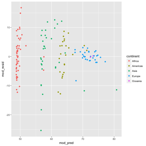
Now that we have augmented the data with predicted values and residuals from the model we can plot those values to better understand what our model says about our data. For example we can inspect a scatter plot of the residuals versus predicted values to see if there are trends in the residuals:

ggplot(gapminder77, aes(x = mod_pred, y = mod_resid, color = continent)) +
  geom_point()

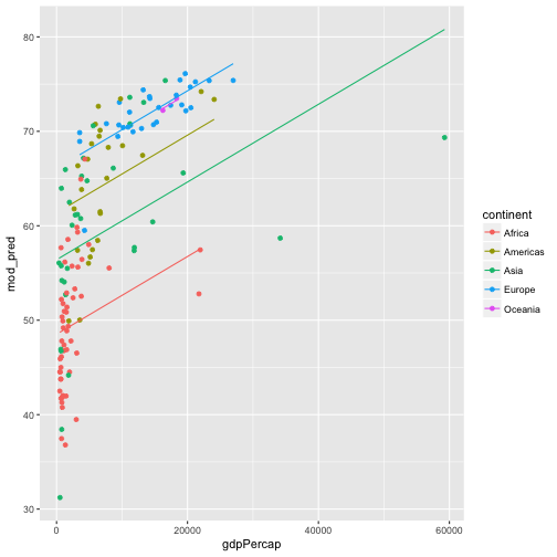
and we can plot the predicted values from out model:

ggplot(gapminder77, aes(x = gdpPercap, y = mod_pred, color = continent)) +
  geom_point(aes(y = lifeExp)) +
  geom_line()

glm and beyond

Finally, the specification of generalized linear models such as logistic or Poisson regressions is very similar via the glm command. See ?glm and the web for help. Beyond glm’s, the statistical capabilities of R are extensive. Recommended packages and functions orgainized by topic are available at https://cran.r-project.org/web/views/. The Social Sciences task view at https://cran.r-project.org/web/views/SocialSciences.html is a good place to start looking for model-fitting function recommendations.