R for reproducible scientific analysis
Manipulating data.frames
Learning objectives
- Be able to use the six major dplyr verbs (
filter,select,arrange,mutate,group_by,summarize) - Be able to use and understand the advantages of the
magrittrpipe:%>%
It is an often bemoaned fact that a data scientist spends much, and often most, of her time wrangling data: getting it organized and clean. In this lesson we will learn an efficient set of tools that can handle the vast majority of most data management tasks.
Enter dplyr, a package for making data manipulation easier. More on dplyr later. dplyr is part of tidyverse, so it is already installed on your machine. You can load it individually, or with the other tidyverse packages like this:
library(tidyverse)Loading tidyverse: ggplot2
Loading tidyverse: tibble
Loading tidyverse: tidyr
Loading tidyverse: readr
Loading tidyverse: purrr
Loading tidyverse: dplyr
Conflicts with tidy packages ----------------------------------------------
filter(): dplyr, stats
lag():    dplyr, stats
Those messages and conflicts are normal. The conflicts are R telling you that there are two packages with functions named “filter” and “lag”. When R gives you red text, it’s not always a bad thing, but it does mean you should pay attention and try to understand what it’s trying to tell you.
Remember that you only have to install each package once (per computer), but you have to load them for each R session in which you want to use them.
You also have to load any data you want to use each time you start a new R session. So, if it’s not already loaded, read in the gapminder data. We’re going to use tidyverse’s read_csv instead of base R’s read.csv here. It has a few nice features; the most obvious is that it makes a special kind of data.frame that only prints the first ten rows instead of all 1704.
gapminder <- read_csv('data/gapminder-FiveYearData.csv')
class(gapminder)
[1] "tbl_df" "tbl" "data.frame"
gapminder# A tibble: 1,704 × 6
country year pop continent lifeExp gdpPercap
<chr> <int> <dbl> <chr> <dbl> <dbl>
1 Afghanistan 1952 8425333 Asia 28.801 779.4453
2 Afghanistan 1957 9240934 Asia 30.332 820.8530
3 Afghanistan 1962 10267083 Asia 31.997 853.1007
4 Afghanistan 1967 11537966 Asia 34.020 836.1971
5 Afghanistan 1972 13079460 Asia 36.088 739.9811
6 Afghanistan 1977 14880372 Asia 38.438 786.1134
7 Afghanistan 1982 12881816 Asia 39.854 978.0114
8 Afghanistan 1987 13867957 Asia 40.822 852.3959
9 Afghanistan 1992 16317921 Asia 41.674 649.3414
10 Afghanistan 1997 22227415 Asia 41.763 635.3414
# ... with 1,694 more rows
You can always convert a data.frame into this special kind of data.frame like this:
gapminder <- tbl_df(gapminder)What is dplyr?
The package dplyr is a fairly new (2014) package that tries to provide easy tools for the most common data manipulation tasks. It is built to work directly with data frames. The thinking behind it was largely inspired by the package plyr which has been in use for some time but suffered from being slow in some cases.dplyr addresses this by porting much of the computation to C++. An additional feature is the ability to work with data stored directly in an external database. The benefits of doing this are that the data can be managed natively in a relational database, queries can be conducted on that database, and only the results of the query returned.
This addresses a common problem with R in that all operations are conducted in memory and thus the amount of data you can work with is limited by available memory. The database connections essentially remove that limitation in that you can have a database of many 100s GB, conduct queries on it directly and pull back just what you need for analysis in R.
The five tasks of dplyr
There are five actions we often want to apply to a tabular dataset:
- Filter rows
- Filter columns
- Arrange rows
- Make new columns
- Summarize groups
We are about to see how to do each of those things using the dplyr package. Everything we’re going to learn to do can also be done using “base R”, but dplyr makes it easier, and the syntax is consistent, and it actually makes the computations faster.
filter()
Suppose we want to see just the gapminder data for the USA. First, we need to know how “USA” is written in the dataset: Is it USA or United States or what? We can see all the unique values of a variable with the unique function.
unique(gapminder$country) [1] "Afghanistan" "Albania"
[3] "Algeria" "Angola"
[5] "Argentina" "Australia"
[7] "Austria" "Bahrain"
[9] "Bangladesh" "Belgium"
[11] "Benin" "Bolivia"
[13] "Bosnia and Herzegovina" "Botswana"
[15] "Brazil" "Bulgaria"
[17] "Burkina Faso" "Burundi"
[19] "Cambodia" "Cameroon"
[21] "Canada" "Central African Republic"
[23] "Chad" "Chile"
[25] "China" "Colombia"
[27] "Comoros" "Congo Dem. Rep."
[29] "Congo Rep." "Costa Rica"
[31] "Cote d'Ivoire" "Croatia"
[33] "Cuba" "Czech Republic"
[35] "Denmark" "Djibouti"
[37] "Dominican Republic" "Ecuador"
[39] "Egypt" "El Salvador"
[41] "Equatorial Guinea" "Eritrea"
[43] "Ethiopia" "Finland"
[45] "France" "Gabon"
[47] "Gambia" "Germany"
[49] "Ghana" "Greece"
[51] "Guatemala" "Guinea"
[53] "Guinea-Bissau" "Haiti"
[55] "Honduras" "Hong Kong China"
[57] "Hungary" "Iceland"
[59] "India" "Indonesia"
[61] "Iran" "Iraq"
[63] "Ireland" "Israel"
[65] "Italy" "Jamaica"
[67] "Japan" "Jordan"
[69] "Kenya" "Korea Dem. Rep."
[71] "Korea Rep." "Kuwait"
[73] "Lebanon" "Lesotho"
[75] "Liberia" "Libya"
[77] "Madagascar" "Malawi"
[79] "Malaysia" "Mali"
[81] "Mauritania" "Mauritius"
[83] "Mexico" "Mongolia"
[85] "Montenegro" "Morocco"
[87] "Mozambique" "Myanmar"
[89] "Namibia" "Nepal"
[91] "Netherlands" "New Zealand"
[93] "Nicaragua" "Niger"
[95] "Nigeria" "Norway"
[97] "Oman" "Pakistan"
[99] "Panama" "Paraguay"
[101] "Peru" "Philippines"
[103] "Poland" "Portugal"
[105] "Puerto Rico" "Reunion"
[107] "Romania" "Rwanda"
[109] "Sao Tome and Principe" "Saudi Arabia"
[111] "Senegal" "Serbia"
[113] "Sierra Leone" "Singapore"
[115] "Slovak Republic" "Slovenia"
[117] "Somalia" "South Africa"
[119] "Spain" "Sri Lanka"
[121] "Sudan" "Swaziland"
[123] "Sweden" "Switzerland"
[125] "Syria" "Taiwan"
[127] "Tanzania" "Thailand"
[129] "Togo" "Trinidad and Tobago"
[131] "Tunisia" "Turkey"
[133] "Uganda" "United Kingdom"
[135] "United States" "Uruguay"
[137] "Venezuela" "Vietnam"
[139] "West Bank and Gaza" "Yemen Rep."
[141] "Zambia" "Zimbabwe"
Okay, now we want to see just the rows of the data.frame where country is “United States”. The syntax for all dplyr functions is the same: The first argument is the data.frame, the rest of the arguments are whatever you want to do in that data.frame.
filter(gapminder, country == "United States")# A tibble: 12 × 6
country year pop continent lifeExp gdpPercap
<chr> <int> <dbl> <chr> <dbl> <dbl>
1 United States 1952 157553000 Americas 68.440 13990.48
2 United States 1957 171984000 Americas 69.490 14847.13
3 United States 1962 186538000 Americas 70.210 16173.15
4 United States 1967 198712000 Americas 70.760 19530.37
5 United States 1972 209896000 Americas 71.340 21806.04
6 United States 1977 220239000 Americas 73.380 24072.63
7 United States 1982 232187835 Americas 74.650 25009.56
8 United States 1987 242803533 Americas 75.020 29884.35
9 United States 1992 256894189 Americas 76.090 32003.93
10 United States 1997 272911760 Americas 76.810 35767.43
11 United States 2002 287675526 Americas 77.310 39097.10
12 United States 2007 301139947 Americas 78.242 42951.65
We can also apply multiple conditions, e.g. the US after 2000:
filter(gapminder, country == "United States" & year > 2000)# A tibble: 2 × 6
country year pop continent lifeExp gdpPercap
<chr> <int> <dbl> <chr> <dbl> <dbl>
1 United States 2002 287675526 Americas 77.310 39097.10
2 United States 2007 301139947 Americas 78.242 42951.65
We can also use “or” conditions with the vertical pipe: |. Notice that the variable (column) names don’t go in quotes, but values of character variables do.
filter(gapminder, country == "United States" | country == "Mexico")# A tibble: 24 × 6
country year pop continent lifeExp gdpPercap
<chr> <int> <dbl> <chr> <dbl> <dbl>
1 Mexico 1952 30144317 Americas 50.789 3478.126
2 Mexico 1957 35015548 Americas 55.190 4131.547
3 Mexico 1962 41121485 Americas 58.299 4581.609
4 Mexico 1967 47995559 Americas 60.110 5754.734
5 Mexico 1972 55984294 Americas 62.361 6809.407
6 Mexico 1977 63759976 Americas 65.032 7674.929
7 Mexico 1982 71640904 Americas 67.405 9611.148
8 Mexico 1987 80122492 Americas 69.498 8688.156
9 Mexico 1992 88111030 Americas 71.455 9472.384
10 Mexico 1997 95895146 Americas 73.670 9767.298
# ... with 14 more rows
A good, handy reference list for the operators (and, or, etc) can be found here.
select()
filter returned a subset of the data.frame’s rows. select returns a subset of the data.frame’s columns.
Suppose we only want to see country and life expectancy.
select(gapminder, country, lifeExp)We can choose which columns we don’t want
select(gapminder, -continent, income = gdpPercap)# A tibble: 1,704 × 5
country year pop lifeExp income
<chr> <int> <dbl> <dbl> <dbl>
1 Afghanistan 1952 8425333 28.801 779.4453
2 Afghanistan 1957 9240934 30.332 820.8530
3 Afghanistan 1962 10267083 31.997 853.1007
4 Afghanistan 1967 11537966 34.020 836.1971
5 Afghanistan 1972 13079460 36.088 739.9811
6 Afghanistan 1977 14880372 38.438 786.1134
7 Afghanistan 1982 12881816 39.854 978.0114
8 Afghanistan 1987 13867957 40.822 852.3959
9 Afghanistan 1992 16317921 41.674 649.3414
10 Afghanistan 1997 22227415 41.763 635.3414
# ... with 1,694 more rows
And we can rename columns
select(gapminder, ThePlace = country, HowLongTheyLive = lifeExp)# A tibble: 1,704 × 2
ThePlace HowLongTheyLive
<chr> <dbl>
1 Afghanistan 28.801
2 Afghanistan 30.332
3 Afghanistan 31.997
4 Afghanistan 34.020
5 Afghanistan 36.088
6 Afghanistan 38.438
7 Afghanistan 39.854
8 Afghanistan 40.822
9 Afghanistan 41.674
10 Afghanistan 41.763
# ... with 1,694 more rows
As usual, R isn’t saving any of these outputs; just printing them to the screen. If we want to keep them around, we need to assign them to a variable.
justUS = filter(gapminder, country == "United States")
USdata = select(justUS, -country, -continent)
USdata
# A tibble: 12 × 4
year pop lifeExp gdpPercap
<int> <dbl> <dbl> <dbl>
1 1952 157553000 68.440 13990.48
2 1957 171984000 69.490 14847.13
3 1962 186538000 70.210 16173.15
4 1967 198712000 70.760 19530.37
5 1972 209896000 71.340 21806.04
6 1977 220239000 73.380 24072.63
7 1982 232187835 74.650 25009.56
8 1987 242803533 75.020 29884.35
9 1992 256894189 76.090 32003.93
10 1997 272911760 76.810 35767.43
11 2002 287675526 77.310 39097.10
12 2007 301139947 78.242 42951.65
Subsetting
- Subset the gapminder data to only Oceania countries post-1980.
- Remove the continent column
- Make a scatter plot of gdpPercap vs. population colored by country
Advanced How would you determine the median population for the North American countries between 1970 and 1980?
Bonus This can be done using base R’s subsetting, but this class doesn’t teach how. Do the original challenge without the filter and select functions. Feel free to consult Google, helpfiles, etc. to figure out how.
arrange()
You can order the rows of a data.frame by a variable using arrange. Suppose we want to see the most populous countries:
arrange(gapminder, pop)# A tibble: 1,704 × 6
country year pop continent lifeExp gdpPercap
<chr> <int> <dbl> <chr> <dbl> <dbl>
1 Sao Tome and Principe 1952 60011 Africa 46.471 879.5836
2 Sao Tome and Principe 1957 61325 Africa 48.945 860.7369
3 Djibouti 1952 63149 Africa 34.812 2669.5295
4 Sao Tome and Principe 1962 65345 Africa 51.893 1071.5511
5 Sao Tome and Principe 1967 70787 Africa 54.425 1384.8406
6 Djibouti 1957 71851 Africa 37.328 2864.9691
7 Sao Tome and Principe 1972 76595 Africa 56.480 1532.9853
8 Sao Tome and Principe 1977 86796 Africa 58.550 1737.5617
9 Djibouti 1962 89898 Africa 39.693 3020.9893
10 Sao Tome and Principe 1982 98593 Africa 60.351 1890.2181
# ... with 1,694 more rows
Hmm, we didn’t get the most populous countries. By default, arrange sorts the variable in increasing order. We could see the most populous countries by examining the tail of the last command, or we can sort the data.frame by descending population by wrapping the variable in desc():
arrange(gapminder, desc(pop))# A tibble: 1,704 × 6
country year pop continent lifeExp gdpPercap
<chr> <int> <dbl> <chr> <dbl> <dbl>
1 China 2007 1318683096 Asia 72.96100 4959.1149
2 China 2002 1280400000 Asia 72.02800 3119.2809
3 China 1997 1230075000 Asia 70.42600 2289.2341
4 China 1992 1164970000 Asia 68.69000 1655.7842
5 India 2007 1110396331 Asia 64.69800 2452.2104
6 China 1987 1084035000 Asia 67.27400 1378.9040
7 India 2002 1034172547 Asia 62.87900 1746.7695
8 China 1982 1000281000 Asia 65.52500 962.4214
9 India 1997 959000000 Asia 61.76500 1458.8174
10 China 1977 943455000 Asia 63.96736 741.2375
# ... with 1,694 more rows
arrange can also sort by multiple variables. It will sort the data.frame by the first variable, and if there are any ties in that variable, they will be sorted by the next variable, and so on. Here we sort from newest to oldest, and within year from richest to poorest:
arrange(gapminder, desc(year), desc(gdpPercap))# A tibble: 1,704 × 6
country year pop continent lifeExp gdpPercap
<chr> <int> <dbl> <chr> <dbl> <dbl>
1 Norway 2007 4627926 Europe 80.196 49357.19
2 Kuwait 2007 2505559 Asia 77.588 47306.99
3 Singapore 2007 4553009 Asia 79.972 47143.18
4 United States 2007 301139947 Americas 78.242 42951.65
5 Ireland 2007 4109086 Europe 78.885 40676.00
6 Hong Kong China 2007 6980412 Asia 82.208 39724.98
7 Switzerland 2007 7554661 Europe 81.701 37506.42
8 Netherlands 2007 16570613 Europe 79.762 36797.93
9 Canada 2007 33390141 Americas 80.653 36319.24
10 Iceland 2007 301931 Europe 81.757 36180.79
# ... with 1,694 more rows
Shoutout Q: Would we get the same output if we switched the order of desc(year) and desc(gdpPercap) in the last line?
mutate()
We have learned how to drop rows, drop columns, and rearrange rows. To make a new column we use the mutate function. As usual, the first argument is a data.frame. The second argument is the name of the new column you want to create, followed by an equal sign, followed by what to put in that column. You can reference other variables in the data.frame, and mutate will treat each row independently. E.g. we can calculate the total GDP of each country in each year by multiplying the per-capita GDP by the population.
mutate(gapminder, total_gdp = gdpPercap * pop)# A tibble: 1,704 × 7
country year pop continent lifeExp gdpPercap total_gdp
<chr> <int> <dbl> <chr> <dbl> <dbl> <dbl>
1 Afghanistan 1952 8425333 Asia 28.801 779.4453 6567086330
2 Afghanistan 1957 9240934 Asia 30.332 820.8530 7585448670
3 Afghanistan 1962 10267083 Asia 31.997 853.1007 8758855797
4 Afghanistan 1967 11537966 Asia 34.020 836.1971 9648014150
5 Afghanistan 1972 13079460 Asia 36.088 739.9811 9678553274
6 Afghanistan 1977 14880372 Asia 38.438 786.1134 11697659231
7 Afghanistan 1982 12881816 Asia 39.854 978.0114 12598563401
8 Afghanistan 1987 13867957 Asia 40.822 852.3959 11820990309
9 Afghanistan 1992 16317921 Asia 41.674 649.3414 10595901589
10 Afghanistan 1997 22227415 Asia 41.763 635.3414 14121995875
# ... with 1,694 more rows
Shoutout Q: How would we view the highest-total-gdp countries?
Note that didn’t change gapminder: We didn’t assign the output to anything, so it was just printed, with the new column. If we want to modify our gapminder data.frame, we can assign the output of mutate back to the gapminder variable, but be careful doing this – if you make a mistake, you can’t just re-run that line of code, you’ll need to go back to loading the gapminder data.frame.
Also, you can create multiple columns in one call to mutate, even using variables that you just created, separating them with commas:
gapminder = mutate(gapminder,
                   total_gdp = gdpPercap * pop,
                   log_gdp = log10(total_gdp))
MCQ: Data Reduction
Produce a data.frame with only the names, years, and per-capita GDP of countries where per capita gdp is less than a dollar a day sorted from most- to least-recent.
- Tip: The
gdpPercapvariable is annual gdp. You’ll need to adjust. - Tip: For complex tasks, it often helps to use pencil and paper to write/draw/map the various steps needed and how they fit together before writing any code.
What is the annual per-capita gdp, rounded to the nearest dollar, of the first row in the data.frame?
- $278
- $312
- $331
- $339
Advanced: Use dplyr functions and ggplot to plot per-capita GDP versus population for North American countries after 1970. - Once you’ve made the graph, transform both axes to a log10 scale. There are two ways to do this, one by creating new columns in the data frame, and another using functions provided by ggplot to transform the axes. Implement both, in that order. Which do you prefer and why?
C’est ne pas une pipe
Suppose we want to look at all the countries where life expectancy is greater than 80 years, sorted from poorest to richest. First, we filter, then we arrange. We could assign the intermediate data.frame to a variable:
lifeExpGreater80 = filter(gapminder, lifeExp > 80)
(lifeExpGreater80sorted = arrange(lifeExpGreater80, gdpPercap))
# A tibble: 21 × 8
country year pop continent lifeExp gdpPercap
<chr> <int> <dbl> <chr> <dbl> <dbl>
1 New Zealand 2007 4115771 Oceania 80.204 25185.01
2 Israel 2007 6426679 Asia 80.745 25523.28
3 Italy 2002 57926999 Europe 80.240 27968.10
4 Italy 2007 58147733 Europe 80.546 28569.72
5 Japan 2002 127065841 Asia 82.000 28604.59
6 Japan 1997 125956499 Asia 80.690 28816.58
7 Spain 2007 40448191 Europe 80.941 28821.06
8 Sweden 2002 8954175 Europe 80.040 29341.63
9 Hong Kong China 2002 6762476 Asia 81.495 30209.02
10 France 2007 61083916 Europe 80.657 30470.02
# ... with 11 more rows, and 2 more variables: total_gdp <dbl>,
# log_gdp <dbl>
In this case it doesn’t much matter, but we make a whole new data.frame (lifeExpGreater80) and only use it once; that’s a little wasteful of system resources, and it clutters our environment. If the data are large, that can be a big problem.
Or, we could nest each function so that it appears on one line:
arrange(filter(gapminder, lifeExp > 80), gdpPercap)# A tibble: 21 × 8
country year pop continent lifeExp gdpPercap
<chr> <int> <dbl> <chr> <dbl> <dbl>
1 New Zealand 2007 4115771 Oceania 80.204 25185.01
2 Israel 2007 6426679 Asia 80.745 25523.28
3 Italy 2002 57926999 Europe 80.240 27968.10
4 Italy 2007 58147733 Europe 80.546 28569.72
5 Japan 2002 127065841 Asia 82.000 28604.59
6 Japan 1997 125956499 Asia 80.690 28816.58
7 Spain 2007 40448191 Europe 80.941 28821.06
8 Sweden 2002 8954175 Europe 80.040 29341.63
9 Hong Kong China 2002 6762476 Asia 81.495 30209.02
10 France 2007 61083916 Europe 80.657 30470.02
# ... with 11 more rows, and 2 more variables: total_gdp <dbl>,
# log_gdp <dbl>
This would become difficult to read if we are performing a number of operations that would require a repeated nesting. But…
There is a better way, and it makes both writing and reading the code easier. The pipe from the magrittr package (which is automatically installed and loaded with dplyr and tidyverse) takes the output of first line, and plugs it in as the first argument of the next line. Since many tidyverse functions expect a data.frame as the first argument and output a data.frame, this works fluidly.
filter(gapminder, lifeExp > 80) %>%
    arrange(gdpPercap)
# A tibble: 21 × 8
country year pop continent lifeExp gdpPercap
<chr> <int> <dbl> <chr> <dbl> <dbl>
1 New Zealand 2007 4115771 Oceania 80.204 25185.01
2 Israel 2007 6426679 Asia 80.745 25523.28
3 Italy 2002 57926999 Europe 80.240 27968.10
4 Italy 2007 58147733 Europe 80.546 28569.72
5 Japan 2002 127065841 Asia 82.000 28604.59
6 Japan 1997 125956499 Asia 80.690 28816.58
7 Spain 2007 40448191 Europe 80.941 28821.06
8 Sweden 2002 8954175 Europe 80.040 29341.63
9 Hong Kong China 2002 6762476 Asia 81.495 30209.02
10 France 2007 61083916 Europe 80.657 30470.02
# ... with 11 more rows, and 2 more variables: total_gdp <dbl>,
# log_gdp <dbl>
To demonstrate how it works, here are some examples where it’s unnecessary.
4 %>% sqrt()[1] 2
2 ^ 2 %>% sum(1)[1] 5
Whatever goes through the pipe becomes the first argument of the function after the pipe. This is convenient, because all dplyr functions produce a data.frame as their output and take a data.frame as the first argument. Since R ignores white-space, we can put each function on a new line, which RStudio will automatically indent, making everything easy to read. Now each line represents a step in a sequential operation. You can read this as “Take the gapminder data.frame, filter to the rows where lifeExp is greater than 80, and arrange by gdpPercap.”
gapminder %>%
    filter(lifeExp > 80) %>%
    arrange(gdpPercap)
# A tibble: 21 × 8
country year pop continent lifeExp gdpPercap
<chr> <int> <dbl> <chr> <dbl> <dbl>
1 New Zealand 2007 4115771 Oceania 80.204 25185.01
2 Israel 2007 6426679 Asia 80.745 25523.28
3 Italy 2002 57926999 Europe 80.240 27968.10
4 Italy 2007 58147733 Europe 80.546 28569.72
5 Japan 2002 127065841 Asia 82.000 28604.59
6 Japan 1997 125956499 Asia 80.690 28816.58
7 Spain 2007 40448191 Europe 80.941 28821.06
8 Sweden 2002 8954175 Europe 80.040 29341.63
9 Hong Kong China 2002 6762476 Asia 81.495 30209.02
10 France 2007 61083916 Europe 80.657 30470.02
# ... with 11 more rows, and 2 more variables: total_gdp <dbl>,
# log_gdp <dbl>
Making your code easier for humans to read will save you lots of time. The human reading it is usually future-you, and operations that seem simple when you’re writing them will look like gibberish when you’re three weeks removed from them, let alone three months or three years or another person. Make your code as easy to read as possible by using the pipe where appropriate, leaving white space, using descriptive variable names, being consistent with spacing and naming, and liberally commenting code.
Challenge: Data Reduction with Pipes
Copy the code you (or the instructor) wrote to solve the previous MCQ Data Reduction challenge. Rewrite it using pipes (i.e. no assignment and no nested functions)
summarize()
Often we want to calculate a new variable, but rather than keeping each row as an independent observation, we want to group observations together to calculate some summary statistic. To do this we need two functions, one to do the grouping and one to calculate the summary statistic: group_by and summarize. By itself group_by doesn’t change a data.frame; it just sets up the grouping. summarize then goes over each group in the data.frame and does whatever calculation you want. E.g. suppose we want the average global gdp for each year. While we’re at it, let’s calculate the mean and median and see how they differ.
gapminder %>%
    group_by(year) %>%
    summarize(mean_gdp = mean(gdpPercap), median_gdp = median(gdpPercap))
# A tibble: 12 × 3
year mean_gdp median_gdp
<int> <dbl> <dbl>
1 1952 3725.276 1968.528
2 1957 4299.408 2173.220
3 1962 4725.812 2335.440
4 1967 5483.653 2678.335
5 1972 6770.083 3339.129
6 1977 7313.166 3798.609
7 1982 7518.902 4216.228
8 1987 7900.920 4280.300
9 1992 8158.609 4386.086
10 1997 9090.175 4781.825
11 2002 9917.848 5319.805
12 2007 11680.072 6124.371
Shoutout Q: Note that summarize eliminates any other columns. Why? What else can it do? E.g. What country should it list for the year 1952!?
There are several different summary statistics that can be generated from our data. The R base package provides many built-in functions such as mean, median, min, max, and range. By default, all R functions operating on vectors that contains missing data will return NA. It’s a way to make sure that users know they have missing data, and make a conscious decision on how to deal with it. When dealing with simple statistics like the mean, the easiest way to ignore NA (the missing data) is to use na.rm=TRUE (rm stands for remove). An alternate option is to use the function is.na(), which evaluates to true if the value passed to it is not a number. This function is more useful as a part of a filter, where you can filter out everything that is not a number. For that purpose you would do something like
gapminder %>%
  filter(!is.na(someColumn))
The ! symbol negates it, so we’re asking for everything that is not an NA.
We often want to calculate the number of entries within a group. E.g. we might wonder if our dataset is balanced by country. We can do this with the n() function, or dplyr provides a count function as a convenience:
gapminder %>%
    group_by(country) %>%
    summarize(number_entries = n())
# A tibble: 142 × 2
country number_entries
<chr> <int>
1 Afghanistan 12
2 Albania 12
3 Algeria 12
4 Angola 12
5 Argentina 12
6 Australia 12
7 Austria 12
8 Bahrain 12
9 Bangladesh 12
10 Belgium 12
# ... with 132 more rows
count(gapminder, country)# A tibble: 142 × 2
country n
<chr> <int>
1 Afghanistan 12
2 Albania 12
3 Algeria 12
4 Angola 12
5 Argentina 12
6 Australia 12
7 Austria 12
8 Bahrain 12
9 Bangladesh 12
10 Belgium 12
# ... with 132 more rows
We can also do multiple groupings. Suppose we want the maximum life expectancy in each continent for each year. We group by continent and year and calculate the maximum with the max function:
gapminder %>%
    group_by(continent, year) %>%
    summarize(longest_life = max(lifeExp))
Source: local data frame [60 x 3]
Groups: continent [?]
continent year longest_life
<chr> <int> <dbl>
1 Africa 1952 52.724
2 Africa 1957 58.089
3 Africa 1962 60.246
4 Africa 1967 61.557
5 Africa 1972 64.274
6 Africa 1977 67.064
7 Africa 1982 69.885
8 Africa 1987 71.913
9 Africa 1992 73.615
10 Africa 1997 74.772
# ... with 50 more rows
Hmm, we got the longest life expectancy for each continent-year, but we didn’t get the country. To get the country, we have to ask R “Where lifeExp is at a maximum, what is the entry in country?” For that we use the which.max function. max returns the maximum value; which.max returns the location of the maximum value.
max(c(1, 7, 4))[1] 7
which.max(c(1, 7, 4))[1] 2
Now, back to the question: Where lifeExp is at a maximum, what is the entry in country?
gapminder %>%
    group_by(continent, year) %>%
    summarize(longest_life = max(lifeExp), country = country[which.max(lifeExp)])
Source: local data frame [60 x 4]
Groups: continent [?]
continent year longest_life country
<chr> <int> <dbl> <chr>
1 Africa 1952 52.724 Reunion
2 Africa 1957 58.089 Mauritius
3 Africa 1962 60.246 Mauritius
4 Africa 1967 61.557 Mauritius
5 Africa 1972 64.274 Reunion
6 Africa 1977 67.064 Reunion
7 Africa 1982 69.885 Reunion
8 Africa 1987 71.913 Reunion
9 Africa 1992 73.615 Reunion
10 Africa 1997 74.772 Reunion
# ... with 50 more rows
Challenge – Part 1
- Calculate a new column: the total GDP of each country in each year.
- Calculate the variance –
var()of countries’ gdps in each year. - Is country-level GDP getting more or less equal over time?
- Plot your findings.
Challenge – Part 2
- Modify the code you just wrote to calculate the variance in both country-level GDP and per-capita GDP.
- Do both measures support the conclusion you arrived at above?
Challenge – Part 3 (Advanced)
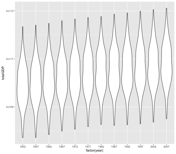
The above plotting exercise asked you to plot summarized information, but it is generally preferable to avoid summarizing before plotting. Can you generate a plot that shows the information you calculated in Part 1 without summarizing?
- Hint:
ggplotinterprets thegapminder$yearas a numeric variable, which may be okay, but there are some plot types for which you needggplotto seegapminder$yearas a category. You can accomplish this by wrapping it infactor– e.g.ggplot(gapminder, aes(x = factor(year) ...
Resources
That is the core of dplyr’s functionality, but it does more. RStudio makes a great cheatsheet that covers all the dplyr functions we just learned, plus what we will learn in the next lesson: keeping data tidy.
Challenge solutions
Solution to challenge Subsetting
- Subset the gapminder data to only Oceania countries post-1980.
- Remove the continent column
- Make a scatter plot of gdpPercap vs. population colored by country
oc1980 = filter(gapminder, continent == "Oceania" & year > 1980)
oc1980less = select(oc1980, -continent)
library('ggplot2')
ggplot(oc1980less, aes(x = gdpPercap, y = lifeExp, color = country)) +
  geom_point()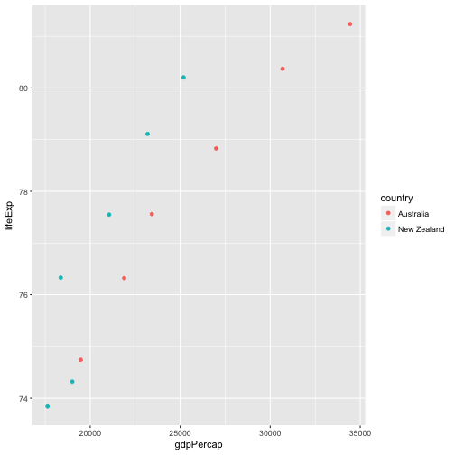
Advanced How would you determine the median population for the North American countries between 1970 and 1980?
noAm = filter(gapminder, country == "United States" |
                country == "Canada" | country == "Mexico" |
                country == "Puerto Rico" & (year > 1970 & year < 1980)
              )
noAmPop = select(noAm, pop)
median(noAmPop)
Error in median.default(noAmPop): need numeric data
noAmPop# A tibble: 38 × 1
pop
<dbl>
1 14785584
2 17010154
3 18985849
4 20819767
5 22284500
6 23796400
7 25201900
8 26549700
9 28523502
10 30305843
# ... with 28 more rows
as.integer(noAmPop)Error in eval(expr, envir, enclos): (list) object cannot be coerced to type 'integer'
median(unlist(noAmPop))[1] 59872135
Bonus This can be done using base R’s subsetting, but this class doesn’t teach how. Do the original challenge without the filter and select functions. Feel free to consult Google, helpfiles, etc. to figure out how.
noAm2 = gapminder[(gapminder$country == "United States") |
                    (gapminder$country == "Mexico") |
                    (gapminder$country == "Canada") |
                    (gapminder$country == "Puerto Rico") &
                    ((gapminder$year > 1970) &
                    (gapminder$year < 1980)),]
median(noAm2$pop)
[1] 59872135
Solution to challenge MCQ: Data Reduction
Produce a data.frame with only the names, years, and per-capita GDP of countries where per capita gdp is less than a dollar a day sorted from most- to least-recent.
- Tip: The
gdpPercapvariable is annual gdp. You’ll need to adjust. - Tip: For complex tasks, it often helps to use pencil and paper to write/draw/map the various steps needed and how they fit together before writing any code.
What is the annual per-capita gdp, rounded to the nearest dollar, of the first row in the data.frame?
- $278
- $312
- $331
- $339
dailyGDP = mutate(gapminder, onedayGDP = gdpPercap / 365)
dailyGDP = filter(dailyGDP, onedayGDP < 1)
dailyGDP = select(dailyGDP, country, year, gdpPercap)
dailyGDP[1,]
# A tibble: 1 × 3
country year gdpPercap
<chr> <int> <dbl>
1 Burundi 1952 339.2965
Advanced: Use dplyr functions and ggplot to plot per-capita GDP versus population for North American countries after 1970. - Once you’ve made the graph, transform both axes to a log10 scale. There are two ways to do this, one by creating new columns in the data frame, and another using functions provided by ggplot to transform the axes. Implement both, in that order. Which do you prefer and why?
noAm = filter(gapminder, country == "United States" |
                country == "Canada" | country == "Mexico" |
                country == "Puerto Rico" & year > 1970
              )
ggplot(noAm, aes(x = gdpPercap, y = pop, color = country)) +
  geom_point() +
  scale_x_log10() +
  scale_y_log10()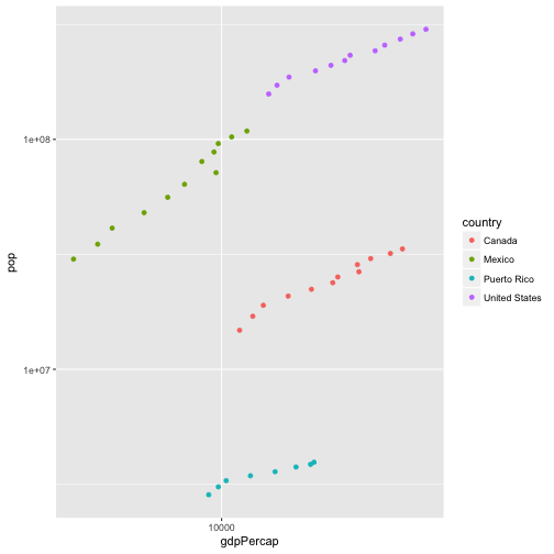
# OR
noAmlog10 = mutate(noAm, log10pop = log10(pop),
                   log10gdp = log10(gdpPercap))
ggplot(noAmlog10, aes(x = log10gdp, y = log10pop, color = country)) +
  geom_point()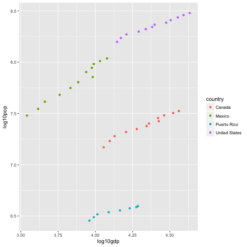
Challenge: Data Reduction with Pipes
Copy the code you (or the instructor) wrote to solve the previous MCQ Data Reduction challenge. Rewrite it using pipes (i.e. no assignment and no nested functions)
# previous challenge with pipes
dailyGDP = mutate(gapminder, onedayGDP = gdpPercap / 365)
dailyGDP = filter(dailyGDP, onedayGDP < 1)
dailyGDP = select(dailyGDP, country, year, gdpPercap)
# BECOMES
smallGDP = gapminder %>%
  mutate(onedayGDP = gdpPercap / 365) %>%
  filter(onedayGDP < 1) %>%
  select(country, year, gdpPercap)
smallGDP[1,]
# A tibble: 1 × 3
country year gdpPercap
<chr> <int> <dbl>
1 Burundi 1952 339.2965
# OR, more fancy (without an intermediate temp variable)
(gapminder %>%
  mutate(onedayGDP = gdpPercap / 365) %>%
  filter(onedayGDP < 1) %>%
  select(country, year, gdpPercap))[1,]
# A tibble: 1 × 3
country year gdpPercap
<chr> <int> <dbl>
1 Burundi 1952 339.2965
Challenge – Part 1
- Calculate a new column: the total GDP of each country in each year.
- Calculate the variance –
var()of countries’ gdps in each year. - Is country-level GDP getting more or less equal over time?
- Plot your findings.
varGDP = gapminder %>%
  mutate(totalGDP = gdpPercap * pop) %>%
  group_by(year) %>%
  summarize(varTotGDP = var(totalGDP))
ggplot(varGDP, aes(x = year, y = varTotGDP)) +
  geom_point()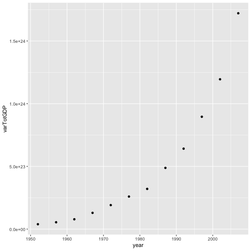
Challenge – Part 2
- Modify the code you just wrote to calculate the variance in both country-level GDP and per-capita GDP.
- Do both measures support the conclusion you arrived at above?
varGDP = gapminder %>%
  mutate(totalGDP = gdpPercap * pop) %>%
  group_by(year) %>%
  summarize(varTotGDP = var(totalGDP),
            varPerCapGDP = var(gdpPercap)
            )
ggplot(varGDP) +
  geom_point(color = "red", aes(x = year, y = varTotGDP)) +
  geom_point(color = "blue", aes(x = year, y = varPerCapGDP))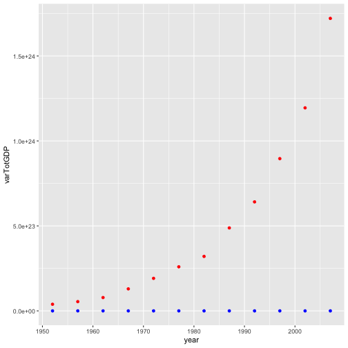
Challenge – Part 3 (Advanced)
The above plotting exercise asked you to plot summarized information, but it is generally preferable to avoid summarizing before plotting. Can you generate a plot that shows the information you calculated in Part 1 without summarizing?
- Hint:
ggplotinterprets thegapminder$yearas a numeric variable, which may be okay, but there are some plot types for which you needggplotto seegapminder$yearas a category. You can accomplish this by wrapping it infactor– e.g.ggplot(gapminder, aes(x = factor(year) ...
gapminder %>%
  mutate(totalGDP = gdpPercap * pop) %>%
ggplot(aes(x = factor(year), y = totalGDP)) +
  geom_violin() +
scale_y_log10() 